15. Dynamic Flux Balance Analysis (dFBA) in COBRApy#
The following notebook shows a simple, but slow example of implementing dFBA using COBRApy and scipy.integrate.solve_ivp. This notebook shows a static optimization approach (SOA) implementation and should not be considered production ready.
The model considers only basic Michaelis-Menten limited growth on glucose.
[1]:
import numpy as np
from tqdm import tqdm

from scipy.integrate import solve_ivp

import matplotlib.pyplot as plt
%matplotlib inline
Create or load a cobrapy model. Here, we use the ‘textbook’ e-coli core model.
[2]:
import cobra
from cobra.io import load_model
model = load_model('textbook')
Scaling...
 A: min|aij| =  1.000e+00  max|aij| =  1.000e+00  ratio =  1.000e+00
Problem data seem to be well scaled
15.1. Set up the dynamic system#
Dynamic flux balance analysis couples a dynamic system in external cellular concentrations to a pseudo-steady state metabolic model.
In this notebook, we define the function add_dynamic_bounds(model, y) to convert the external metabolite concentrations into bounds on the boundary fluxes in the metabolic model.
[3]:
def add_dynamic_bounds(model, y):
    """Use external concentrations to bound the uptake flux of glucose."""
    biomass, glucose = y  # expand the boundary species
    glucose_max_import = -10 * glucose / (5 + glucose)
    model.reactions.EX_glc__D_e.lower_bound = glucose_max_import


def dynamic_system(t, y):
    """Calculate the time derivative of external species."""

    biomass, glucose = y  # expand the boundary species

    # Calculate the specific exchanges fluxes at the given external concentrations.
    with model:
        add_dynamic_bounds(model, y)

        cobra.util.add_lp_feasibility(model)
        feasibility = cobra.util.fix_objective_as_constraint(model)
        lex_constraints = cobra.util.add_lexicographic_constraints(
            model, ['Biomass_Ecoli_core', 'EX_glc__D_e'], ['max', 'max'])

    # Since the calculated fluxes are specific rates, we multiply them by the
    # biomass concentration to get the bulk exchange rates.
    fluxes = lex_constraints.values
    fluxes *= biomass

    # This implementation is **not** efficient, so I display the current
    # simulation time using a progress bar.
    if dynamic_system.pbar is not None:
        dynamic_system.pbar.update(1)
        dynamic_system.pbar.set_description('t = {:.3f}'.format(t))

    return fluxes

dynamic_system.pbar = None


def infeasible_event(t, y):
    """
    Determine solution feasibility.

    Avoiding infeasible solutions is handled by solve_ivp's built-in event detection.
    This function re-solves the LP to determine whether or not the solution is feasible
    (and if not, how far it is from feasibility). When the sign of this function changes
    from -epsilon to positive, we know the solution is no longer feasible.

    """

    with model:

        add_dynamic_bounds(model, y)

        cobra.util.add_lp_feasibility(model)
        feasibility = cobra.util.fix_objective_as_constraint(model)

    return feasibility - infeasible_event.epsilon

infeasible_event.epsilon = 1E-6
infeasible_event.direction = 1
infeasible_event.terminal = True
15.2. Run the dynamic FBA simulation#
[4]:
ts = np.linspace(0, 15, 100)  # Desired integration resolution and interval
y0 = [0.1, 10]

with tqdm() as pbar:
    dynamic_system.pbar = pbar

    sol = solve_ivp(
        fun=dynamic_system,
        events=[infeasible_event],
        t_span=(ts.min(), ts.max()),
        y0=y0,
        t_eval=ts,
        rtol=1e-6,
        atol=1e-8,
        method='BDF'
    )
t = 5.804: : 185it [00:05, 34.89it/s]
Because the culture runs out of glucose, the simulation terminates early. The exact time of this ‘cell death’ is recorded in sol.t_events.
[5]:
sol
[5]:
  message: 'A termination event occurred.'
     nfev: 179
     njev: 2
      nlu: 14
      sol: None
   status: 1
  success: True
        t: array([0.        , 0.15151515, 0.3030303 , 0.45454545, 0.60606061,
       0.75757576, 0.90909091, 1.06060606, 1.21212121, 1.36363636,
       1.51515152, 1.66666667, 1.81818182, 1.96969697, 2.12121212,
       2.27272727, 2.42424242, 2.57575758, 2.72727273, 2.87878788,
       3.03030303, 3.18181818, 3.33333333, 3.48484848, 3.63636364,
       3.78787879, 3.93939394, 4.09090909, 4.24242424, 4.39393939,
       4.54545455, 4.6969697 , 4.84848485, 5.        , 5.15151515,
       5.3030303 , 5.45454545, 5.60606061, 5.75757576])
 t_events: [array([5.80191035])]
        y: array([[ 0.1       ,  0.10897602,  0.11871674,  0.12927916,  0.14072254,
         0.15310825,  0.16649936,  0.18095988,  0.19655403,  0.21334507,
         0.23139394,  0.25075753,  0.27148649,  0.29362257,  0.31719545,
         0.34221886,  0.36868605,  0.3965646 ,  0.42579062,  0.4562623 ,
         0.48783322,  0.52030582,  0.55342574,  0.58687742,  0.62028461,
         0.65321433,  0.685188  ,  0.71570065,  0.74425054,  0.77037369,
         0.79368263,  0.81390289,  0.83089676,  0.84467165,  0.85535715,
         0.8631722 ,  0.86843813,  0.8715096 ,  0.8727423 ],
       [10.        ,  9.8947027 ,  9.78040248,  9.65642157,  9.52205334,
         9.37656372,  9.21919615,  9.04917892,  8.86573366,  8.6680879 ,
         8.45549026,  8.22722915,  7.98265735,  7.72122137,  7.442497  ,
         7.14623236,  6.83239879,  6.50124888,  6.15338213,  5.78981735,
         5.41206877,  5.02222068,  4.62299297,  4.21779303,  3.81071525,
         3.40650104,  3.01042208,  2.6280723 ,  2.26504645,  1.92656158,
         1.61703023,  1.33965598,  1.09616507,  0.88670502,  0.70995892,
         0.56344028,  0.44387781,  0.34762375,  0.27100065]])
 y_events: [array([[0.87280538, 0.25178492]])]
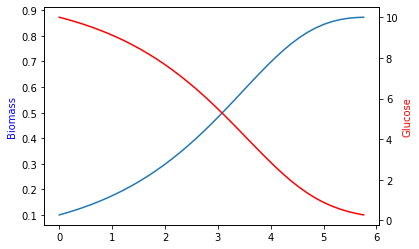
15.2.1. Plot timelines of biomass and glucose#
[6]:
ax = plt.subplot(111)
ax.plot(sol.t, sol.y.T[:, 0])
ax2 = plt.twinx(ax)
ax2.plot(sol.t, sol.y.T[:, 1], color='r')

ax.set_ylabel('Biomass', color='b')
ax2.set_ylabel('Glucose', color='r')
[6]:
Text(0, 0.5, 'Glucose')
[ ]: